Analytic models

Mathematical models of systems

Pros:

• timescales to speed up
• extreme conditions testing
• side effect of gaining clearer understanding of how real system functions

Cons:

• expensive to build/validate/use
• only approx. of real system, edge cases of real system may not be captured.

Purpose: models should be used for trends.

Stochastic Process

Empirical process that changes in time accordining to probabilistic forces.

• Queueing system: QUEUE, SERVE, LEAVE

1. Let $N(t)$, a discrete rv, denote num. jobs at time $t$.
   1. behaviour specification is the pmf
2. Let $W_n$, a continuous rv, denote waiting time of job $n$.
   1. behaviour specification is the pdf

Types

• Markov Processes: $P(state_{now})$
• Birth death processes: $P(state_{now},\ state_{neighbours})$
• Poisson Process: $P(state_{now},\ state_{neighbours}) \wedge Poi(\lambda)$, given
  • inter-arrival times $\tau_j$ have independent and identically distributed mean arrival rates $\lambda$
  • $\tau_j$ are exponentially distributed $\tau \sim \exp(\alpha)$

Poisson process can be split and pooled.

Approaches

1. Queueing theory
   1. Probabilistic job arrivals & service times
   2. state machine
2. Ops analysis:
   1. Measuring averages
   2. Operational quantities

Examples of Performance Questions:

1. What is ave. service time?
2. What is the throughput of the system (num jobs finished over time)
3. If $\lambda \rightarrow 2\lambda$, then how much should $\mu$ increase

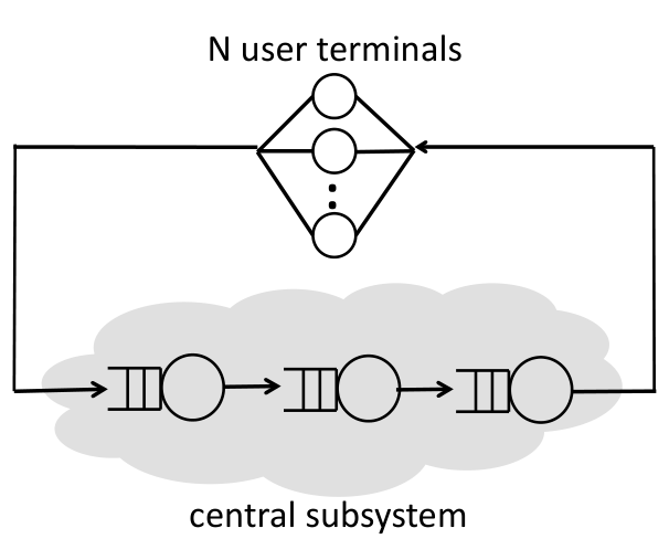
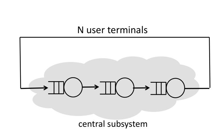
Queueing networks

1. Open: External arrivals/departure
   1. Finite/Infinite job buffer
      1. jobs not in buffer are lost
   2. Network of queues with probabilistic/non-probabilistic routing
      1. do jobs follow a pre-determined route?
      2. the jobs queueing are also in the system
2. Closed: No external arrivals/departures
   1. Interactive/Batch
   2. jobs are issued by a bounded number of users/terminals
   3. jobs are processed by the central subsystem
   4. the user cannot submit a next job before the previous job returns, so the max. number of jobs in the system is fixed
   5. the jobs each user is queueing (if any) are NOT ENERATED/NOT PART OF THE SYSTEM
   6. Think time (Z) a rv for the time between receivign reply from sys and issueing new job.
   7. batch systems circulates in the system without any think time. high throughput.

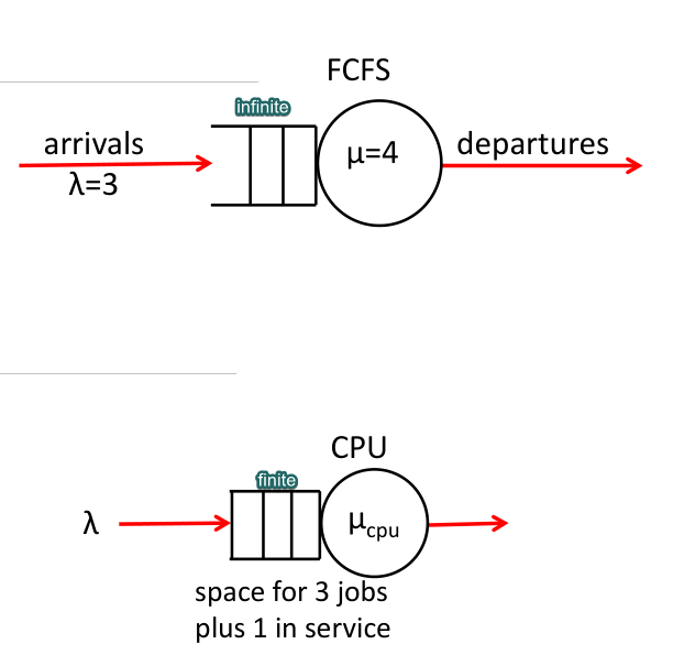
Kendall Notation for queueing network

Note that 1 queue = 1 queuing network.

A/S/m shorthand, A/S/m/B/K/SD full length

• A: interarrival time distribution
  • $D$: deterministic (constant time, no variance)
  • $M$: memoryless (exponential distribution)
  • $E_k$: Erlang-k
  • $H_k$: hyper-exponential $k$ stages
  • $G$: general
• S: Service time distribution
  • Also $D, M, E_k, H_k, G$
• m: number of servers
  • i.e. number of servers this queue is supplying jobs to
• B: system’s capacity (default: $\infty$)
• K: number of customers in source/population size (default: $\infty$)
• SD: Service Discipline (default: FCFS;)
  • FCFS
  • Round Robin (RR)
  • Processor Sharing
  • Shortest Processing Time

Summary of the RVs

Service Time:

• $t_j$: arrival epoch of job $j$
• $\tau_j = t_j - t_{j-1}$: interarrival time
• $\lambda$ mean arrival rate
• $s$: service time per job
• $\mu$: mean service rate per server
• $m$: number of servers

Number of Jobs

• $n_q$: number of queuing jobs
• $n_s$: number of jobs being serviced
• $n = n_q + n_s$
• $E[n] = E[n_q] + E[n_s]$

Response Time:

• $w$: waiting time in queue
• $s$: service time
• $r = w + s$: response time
• $E[r] = E[w] + E[s]$

Fundamental Rules for Queues

1. STABLE: $\lambda < m\mu$
2. JOB COUNT: $n = n_q + n_s$
3. Little’s Law: $E[n] = \lambda E[r]$
4. TIME: $r = w + s$

Little’s Law

Mean jobs = mean arrival rate * mean response time.

Utilization

Utilization ($0 \leq \rho \leq 1$) is mean arrival rate * mean service time i.e. mean number of jobs in service at any point

$P_0 = \text{probability of servers being idle} = 1 - \rho = 1 - \lambda E[s]$