The contents follow the NUS module CS3241 (taken in AY2021/22 S1).
Given in order of progress.
$\require{color}$
Scene: VOLM (Viewer, object, light source, material)
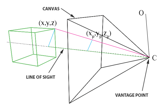
Let $d$ be the distance between the virtual plane and the pinhole. By similar triangles, $x_p = \frac{dx}{z}, y_p = \frac{dy}{z}, z_p = d$.
If $O \neq C$, then for each point $P (x,y,z)$ on the 3D object in the world space, $\overrightarrow{CP}= \overrightarrow{OP} - \overrightarrow{OC}$.
Color: RGB corresponding to visual tristimulus.
API: specifies scene (VOLM), configures/controls the system.
Renderer: produces images using scene info + system config.
Ray-tracing: Following rays of light from $C$ to some point $P$ on objects, or go off into infinity.
Radiosity: Slow, non-general energy based approach
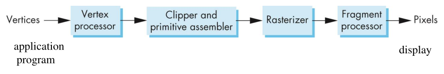
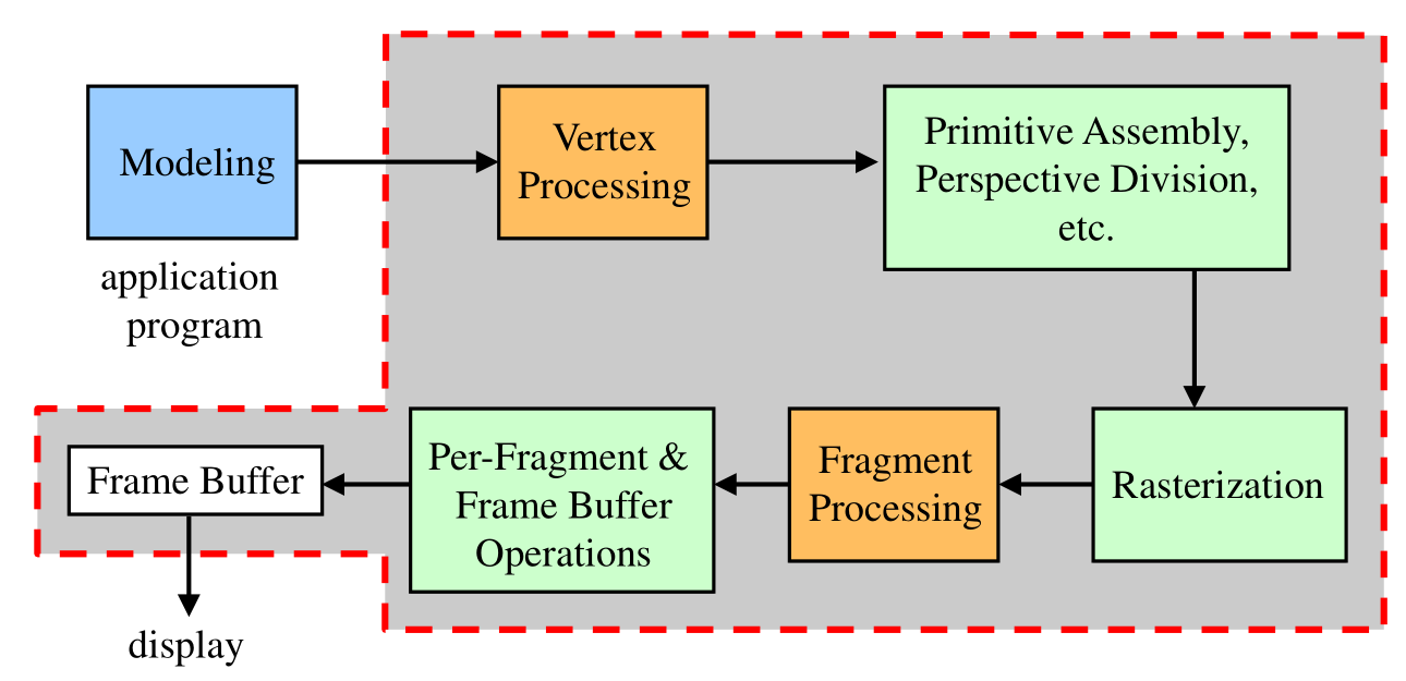
Polygon Rasterization: For each new polygon (primitive) generated, its pixels are assigned.
Objects are meshes of polygonal primitives.
Each primitive is rendered through this pipeline.
The region of memory that holds color and depth data via the attached color and depth buffers.
Required: Functions to specify VOLM, I/O, system capacities (e.g. how many light sources can be supported?)
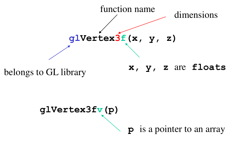
Primitives are defined with vertices.
glBegin(GL_POLYGON)
	glVertex3f(0.0, 0.0, 0.0);
	glVertex3f(0.0, 1.0, 0.0);
	glVertex3f(0.0, 0.0, 1.0);
glEnd();
Camera is specified with
Light source is specified with
Material attributes are
The success of IRIS GL, the graphics API for the world’s first graphics hardware pipeline, led to OpenGL (1992). It’s a platform-independent API.
OpenGL32 on Windows, libGL.a on *nix.Primitive Generation: if primitive is visible, then try output. Appearance depends on the primitive’s state.
State Changing: e.g. Color changing is a state changing function. Changes the “pen color” state to $\textcolor{red}{\textsf{RED}}$ for instance, then it assigns those primitives affected to state $\textcolor{red}{\textsf{RED}}$.
All vectors are represented as a 4D vector by default internally.
Commands are sent to a command queue/buffer.
int main(int argc, char** argv) {
    glutInit(&argc, argv);
    glutInitDisplayMode(GLUT_SINGLE | GLUT_RGB);
    glutInitWindowSize(h, w);
    glutInitWindowPosition(0, 0);
    glutCreateWindow("simple");
    glutDisplayFunc(mydisplay); // mydisplay is the display callback

    init();

    glutMainLoop(); // if anything happens, calls mydisplay to refresh
}
main defines callback, opens windows, enters event loop.init sets state variables (viewing, attributes).void init() {
glClearColor(0.0, 0.0, 0.0, 1.0); // black clear color + opaque window
glColor3f(1.0, 1.0, 1.0); // set fill to white
glMatrixMode(GL_PROJECTION);
glLoadIdentity();
glOrtho(-1.0, 1.0, -1.0, 1.0, -1.0, 1.0); // FOV setting.
// the square is *enclosed* in the FOV.
}
At the beginning, object coordinates = world coordinates. The camera is positioned in world.
Then a viewing volume must be set. It is specified in camera/eye/view coordinates.
Internally OpenGL converts vertices to eye coordinates with GL_MODELVIEW, and then to window coordinates with GL_PROJECTION.
Viewing volume: The finite volume in world space in which objects can be seen. The coordinates are set relative to the camera’s coordinates (eye coordinates).
Projection plane: In OpenGL this is equivalent to the near plane which is always perpendicular to the z axis of the camera coordinate axis. Note: near plane (negative z direction), far plane (positive z direction)
OpenGL only renders Simple, Convex, Flat polygons.
Convex:
glShadeModel(GL_SMOOTH) allows smooth interpolation of colors across the interior of the polygon.
glShadeModel(GL_FLAT) picks one vertex to follow its color
glViewport(x,y,w,h)
Here the order in which polygons are drawn matters, otherwise hidden surface removal would be necessary to prevent surfaces “clipping” through one another.
How do we make a 3D Sierpinski Gasket given the code for a 2D one?
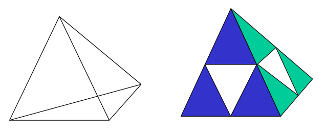
4 different Sierpinski triangles (see reds, blues, blacks and greens).
However the triangles are drawn in the order defined by the program, the black , red and blue triangles may not always be in front of the reds as desired.
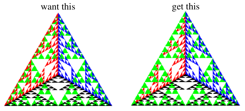
OpenGL now must use HSR via the z-buffer algorithm that saves depth info (via depth buffer, aka z-buffer) as only objects with lowest z-value at that pixel are rendered.
The display loop:
Input Physical properties – Mouse, Keyboard etc. Contains trigger which sends a signal to the OS.
Input Logical properties – What is returned to the program via an API (the measure).
Trigger generates event. Event measure is entered into event queue.
The main programming interface for event-driven input. For each type of event the system recognizes, we define a callback.
e.g. glutMouseFunc(mymouse) means mymouse is set as the mouse callback to handle any mouse clicking.
On each pass of the event loop, for each event in the queue, GLUT calls the callback function if it is defined.
e.g. The display callback is executed whenever window needs to be refreshed.
glutPostRedisplay() when called, sets a flag.To redraw the display, we usually call glClear() first. But the frame buffer is decoupled from the display of the contents when cleared. Partially drawn display will then flicker.
Double buffering:
glutInitDisplayMode(GLUT_RGB | GLUT_DOUBLE) in main()void mydisplay() {
glClear(GL_COLOR_BUFFER_BIT|...) // on the back buffer
/* draw my graphics*/
glutSwapBuffers(); // push the back to the front and front to the back
}
Idle callback: glutIdleFunc(myidle)
void myidle() {
	t += dt
	glutPostRedisplay(); // mark to update image.
}
void mydisplay() { /* draws something that depends on t */}
Note that since the signatures of all GLUT callbacks are fixed, to pass around variables we need to use globals.
glutMotionFunc(...) and glutPassiveMotionFunc(...)glutKeyboardFunc(...)glutReshapeFunc(...): good place to put viewing functions, since it is invoked from window first opening.Template:
void myReshape(int w, int h) {
	glViewport(0, 0, w, h);
	glMatrixMode(GL_PROJECTION);
	glLoadIdentity();
    /* set projection matrix here! */
	glMatrixMode(GL_MODELVIEW);
}
Viewport aspect ratio = Window aspect ratio:
// l, r, b, t are the original left right bottom top coordinates.
if (w <= h)
	gluOrtho2D( l, r, b * (GLfloat) h / w, t * (GLfloat) h / w );
else
	gluOrtho2D( l * (GLfloat) w / h, r * (GLfloat) w / h, b, t );
Resize exactly (clip if necessary):
// l, x, b, y are the original left (right-left) bottom (top-bottom) values.
// This version anchors to the bottom left.
gluOrtho2D( l, l + x * h/origWinWidth, b, b + y * h/origWinHeight );
Affine space. Vector space without a fixed origin. Between 2 points we have a displacement/translation vector.
Frame. Adding a single point to the affine space as an origin.
Note: we only need to transform endpoints of line segments, points on the line segment itself is drawn by the implementation.
| Type | Matrix |
|---|---|
| Translation $T(d_x, d_y, d_z)$ $T^{-1}(v) = T(-v)$ |
$\left[ \matrix{1 & 0 & 0 & d_x \\ 0 & 1 & 0 & d_y \\0 & 0 & 1 & d_z \\ 0 & 0 & 0 & 1} \right]$ |
| Rotation $R_z(\theta)$ $R^{-1}(\theta) = R(-\theta)\\ = R(\theta)^T$ |
$\left[ \matrix{\cos\theta & \sin\theta & 0 & d_x \\ -\sin\theta & \cos\theta & 0 & d_y \\ 0 & 0 & 1 & d_z \\ 0 & 0 & 0 & 1} \right]$ |
| Scaling $S(s_x, s_y, s_z)$ $S^{-1}(v) = S(1/v)$ |
$\left[ \matrix{s_x & 0 & 0 & 0 \\ 0 & s_t & 0 & 0 \\ 0 & 0 & s_z & 0 \\ 0 & 0 & 0 & 1} \right]$ |
| Shear $H(\theta)$ (Note that this shear matrix does $x’ = x+ y\cot\theta$.) |
$\left[ \matrix{1 & \cot\theta & 0 & 0 \\ 0 & 1 & 0 & 0 \\ 0 & 0 & 1 & 0 \\ 0 & 0 & 0 & 1} \right]$ |
Instancing. Starting with a simple object @origin, @original size, we can apply an instance transformation to scale/orientate/locate.
Rotate object about point $p_f$: $M = T(p_f)R(\theta)T(-p_f)$.
Matrix modes. Matrices are part of the state, and matrix modes provide a set of functions for manipulation. GL_MODELVIEW and GL_PROJECTION are two such matrices.
Each mode has a 4x4 homogenous coordinate matrix. The current transformation matrix (CTM) is part of this state and applied to all vertices down this pipeline. $p’ = Cp$ where $C$ is the CTM.
GL_MODELVIEW used to transform objects into world space (also position camera, but gluLookAt does that better). GL_PROJECTION is used to define the view volume.
function (each has double ver. too) |
effect |
|---|---|
glLoadIdentity() |
loads $I$ |
glRotatef(theta, vx, vy, vz) |
post-multiply $R(\theta)$. $[vx, vy, vz]$ are rotation axes |
glTranslatef(dx, dy, dz) |
post-multiply $T(dx, dy, dz)$ |
glScalef(sx, sy, sz) |
post-multiply $S(sx, sy, sz)$ |
glLoadMatrixf(m) |
loads 4x4 matrix $M$ as a float[16] |
glMultMatrixf(m) |
post-multiply $M$. |
glPushMatrix and glPopMatrix...
glPushMatrix();
glRotated(i*45.0, 0.0, 0.0, 1.0); // pushed each of these onto a stack
glTranslated(10.0, 0.0, 0.0);
glScaled(0.5, 0.5, 0.5);
DrawSquare(); // Apply stacked matrix to the element (square)
glPopMatrix(); // Emptied out stack
...
Pose. Position + Orientation. Done by view transformation.
Projection. Orthographic vs Perspective.
Prerequisite: object geometry to be set and placed the world coordinate.
Projectors. lines that either
They preserve lines but not necessarily angles (in the 2D image). Preserving here means that the angles between 2 vectors in the object are the same as that in the image.
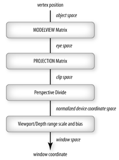
MODELVIEW actually is a combination of the modelling transformation first (to the world space), and the view transformation (to the eye/camera space). PROJECTION matrix brings this to the clip space, and so on.
MODELVIEW matrix is $I$ so initially world frame = camera framePROJECTION matrix is $I$ and orthographic ().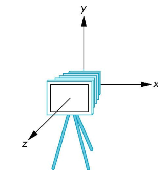
gluLookAt(eyex, eyey, eyez, atx, aty, atz, upx, upy, upz)
eye: origin of camera lens (viewpoint)
at: any point along the viewing direction
up: $y$ axis of the camera
up doesn’t have to be perpendicular to eye - at, as long as $y_c$ can be found by a linear combination of these twoCamera’s coordinate vectors $u, v, n$ are then derived in the $x,y,z$ directions respectively.
So all points in world frame are expressed wrt the camera frame.
(We can use $u, v, n$ directly in $R$ because they are unit vectors in the desired directions)
$M_n = (M_t^{-1})^T$, where $M_t$ is the top left 3x3 submatrix of $M$.
3x3 matrix is enough cos it does not have position (thus $M_n$ would be an affine transformation).
Since rotation matrices are orthogonal, $R^{-1} = R^T$. Thus if $M$ is a rotational matrix, $M_n = M_t$.
Defined with a view (clipping) volume in the camera frame, and is specified in camera space.
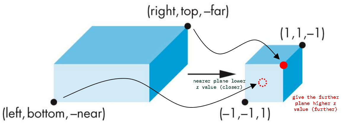
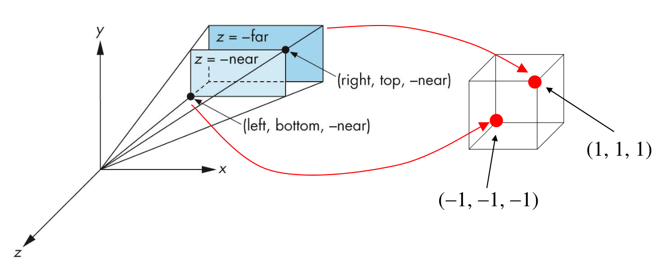
glOrtho(left, right, bottom, top, near, far)glFrustum(left, right bottom, top, near, far)near is in +z direction, and far is in -z direction, but provide near < farThe projection matrix is computed such that it maps to the canonical view volume ($2^3$ cube) in Normalized Device Coordinates (NDC) space. Criteria
At the end of each vertex shader run, OpenGL expects the coordinates to be within a specific range and any coordinate that falls outside this range is clipped. Coordinates that are clipped are discarded, so the remaining coordinates will end up as fragments visible on your screen. This is also where clip space gets its name from.
Source: https://learnopengl.com/Getting-started/Coordinate-Systems
Mapping from $(right,top,-far) \rightarrow (1, 1, 1)$, and $(left,bottom,-near) \rightarrow (-1, -1, -1)$.
The viewport here is defined by $(x_{vp}, y_{vp})$ (the lower left corner), $w,h$.
\[\begin{aligned} \frac{x_{NDC} - (-1)}{2} &= \frac{x_{win} - x_{vp}}{w} \Rightarrow x_{win} = x_{vp} + \frac{w(x_{NDC} + 1)}{2} \\ \frac{y_{NDC} - (-1)}{2} &= \frac{y_{win} - y_{vp}}{h} \Rightarrow y_{win} = y_{vp} + \frac{h(y_{NDC} + 1)}{2} \\ &z_{win} = \frac{z_{NDC} + 1}{2} \end{aligned}\]Squashed into the $x,y$ plane. $z$ is retained (between 0 and 1) for hidden surface removal.
Mapping from $(right,top,-far) \rightarrow (1, 1, 1)$, and $(left,bottom,-near) \rightarrow (-1, -1, -1)$.
Should happen after clipping to prevent any division by zeroes (for a vertex at $z = 0$)
Essentially using similar triangles (as described in first chapter) to get coordinates adjusted for perspective depth. note that $z_p = d$, the projection plane.
\[\begin{aligned} &\frac{x_p}{x} = \frac{d}{z}, \quad \frac{y_p}{y} = \frac{d}{z}, \quad z_p = d \\ \Rightarrow& x_p = \frac{x}{z/d}, x_p = \frac{y}{z/d}, z_p = \frac{z}{z/d} \\ \end{aligned}\]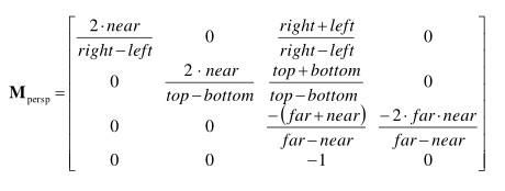
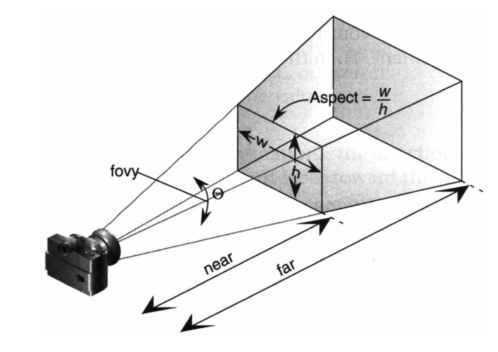
gluPerspective(fovy, aspect, near, far) specifies a symmetric view volume.
Find intersections of 2D line segments with the clipping window.
Eliminate all easy cases without computing intersections.
Outcodes are defined for each area:
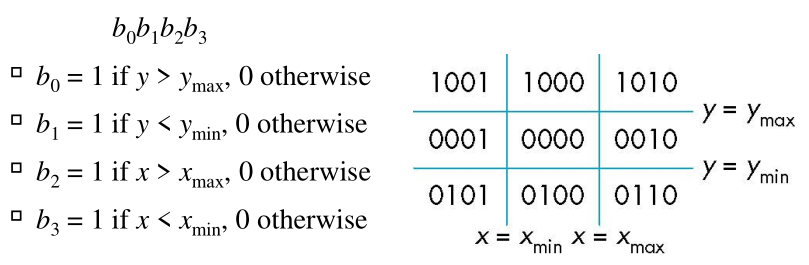
Let $F(A,B)$ represent the clipping requirement of the line segment $AB$. $F(A,B)$ equals 2 if it is not clipped out, 1 if it is partially clipped out, and 0 if it is fully clipped out.
\[F(A, B) = \begin{cases} 2 & A = 0 \text{ and } B = 0 \\ 1 & A = 0 \text{ and } B \neq 0 \\ 0 & A \text{ AND } B \text{ (bitwise)} \neq 0 \\ 1 & A \neq 0 \text{ and } B \neq 0 \text{ and } A \text{ AND } B \text{ (bitwise)} = 0 \end{cases}\]To compute the last case: shorten line segment by intersecting with one of the sides, recursively compute outcode until $A = B = 0$. For 3D, we have 6-bit outcodes ($9 \times 3 = 27$ of them, each prefixed with 00, 01, or 10).
Clip space: After projection matrix, before perspective division.
If vertex $[x_{clip}, y_{clip}, z_{clip}, w_{clip}]$ is in canonical view volume $[-1,1]^3$ after perspective division, we must have $-1 \leq x_{clip} / w_{clip} \leq 1 \Rightarrow -w_{clip} \leq x_{clip} \leq w_{clip}$, and similarly for $y, z$. These define the clipping planes.
| To be clipped | Yields |
|---|---|
| Line segment | 1 |
| General Polygon | $\geq 1$ |
| Convex polygon | 1 |
Hence change polygons to convex polygons (tessellation), commonly using triangulation.
All line segments pass through top clipping, then bottom clipping, and so on until final form. Similar for polygons (with front and back clippers.)
However small increase in latency.
Not implemented in pipeline.
Straight lines $y = mx + b$ satisfies differential equation $\frac{dy}{dx} = \frac{y_e - y_0}{x_e - x_0}$.
Case 1: $0 \leq |m| \leq 1$. Loop through each pixel $(x_i, y_i) = (x_0 + i, y_{i-1} + m)$.
Case 2: $|m| > 1$. Then note that $0 \leq \frac{1}{|m|} \leq 1$. Hence loop through each pixel $(x_i, y_i) = (x_{i-1} + m, y_0 + i)$.
Saves time because of no floating point computations. Let $x_k, y_k$ be the current pixel locations (integers).
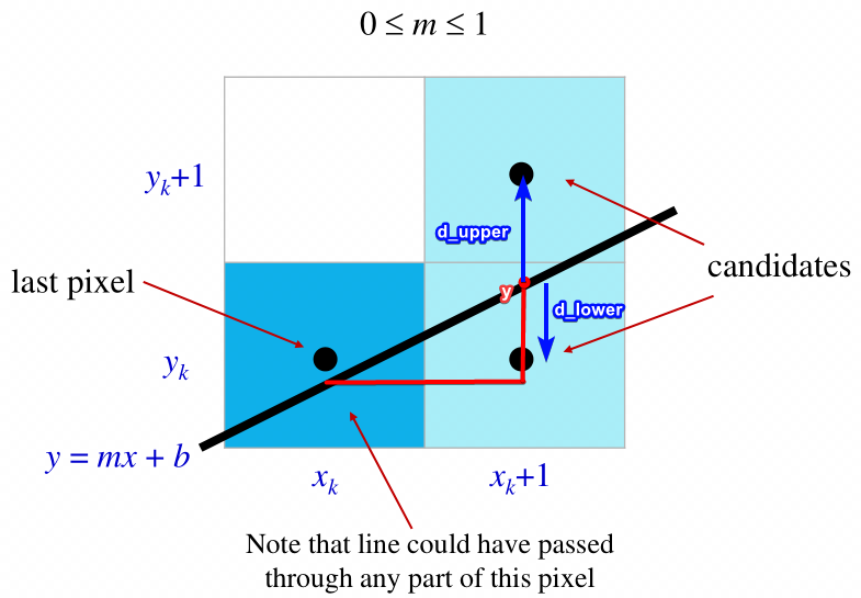
Note that:
Here since $d_{upper} > d_{lower}$, we choose to shade $(x_k + 1, y_k)$.But how does it save FP computation time? Compute decision variable $p_k$ for pixel $k$: If $p_k < 0$ plot lower pixel, if $p_k > 0$ plot upper pixel.
\[\begin{aligned} p_k =& \Delta x(d_{lower} - d_{upper}) \\ =& \Delta x(y - y_k - (y_k+1) + y) \\ =& \Delta x(2y - 2y_k - 1) \\ =& 2x_k \Delta y - 2y_k \Delta x + c' \end{aligned}\]Since $p_{k+1} - p_k = 2(x_{k+1} - x_k)\Delta y + 2(y_{k+1} - y_k)\Delta x$, we have
See Bressenham’s circle algorithm.
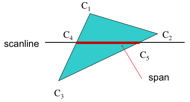
Horizontal scanlines: Get both endpoints by interpolating the line segment they are each on.
from a seed point located inside, scan-convert the edges using edge color (recursively).
flood_fill(int x, int y) {
	if (A[x][y] == WHITE) {
		A[x][y] = BLACK;
		flood_fill(x-1, y);
		flood_fill(x+1, y);
		flood_fill(x, y+1);
		flood_fill(x, y-1);
	}
}
Eliminate back-facing + invisible polygons (e.g. cube only have 3 faces facing viewport at all times. The rest can be culled.) $N_\text{face} \cdot V_\text{camera to vertex} \leq 0$.
In OpenGL, if the vertices on a plane are specified counterclockwise, that face is front-facing.
Can be remedied by reducing the distance between near and far planes in view volume, or increasing the floating point accuracy of the z-buffer.
Given point on surface, light source, viewpoint: compute color of point
Since Gouraud shading is per-vertex, takes place at Vertex Processing stage, in Camera space
glEnable(GL_LIGHTING) enables shading calculations, disables glColor
glEnable(GL_LIGHTi) for $i \in [0 \dots 7]$
glLightModeli(parameter, GL_TRUE)GLfloat[] for each
ambienti, diffusei, specularilighti_pos: if lighti_pos[3] == 1.0: point light. else if == 0.0: directional lightglLightModelfv(GL_LIGHT_MODEL_AMBIENT, global_ambient) sets the global ambient light $I_{ga}$glMaterialfv(GL_FRONT, GL_X, type X)
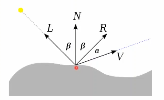
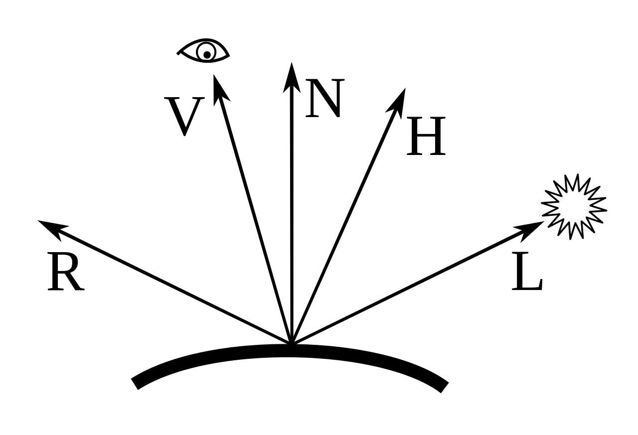
AMBIENT, DIFFUSE, SPECULAR = GLfloat[] i.e. $I_{a,i}, I_{d,i}, I_{s,i}$SHININESS = GLfloatGL_FRONT | GL_BACK | GL_FRONT_AND_BACKEMISSION = GLfloat[] Emissive term $k_e$ (glowing)Efficient, acceptable image quality. Ambient ($I_a k_a$), diffuse ($f_{\text{att}} I_p k_d (N \cdot L)$), and specular ($f_{\text{att}} I_p k_s (R \cdot L)^n$) components. Single light source below:
\[I_{\text{Phong}} = \left[ \begin{matrix} r \\ g \\ a \end{matrix} \right] = I_a k_a + f_{\text{att}} I_p k_d (N \cdot L) + f_{\text{att}} I_p k_s (R \cdot L)^n\]Multiple light sources $L_i$:
\[I_{\text{Phong}} = \left[ \begin{matrix} r \\ g \\ a \end{matrix} \right] = I_a k_a + f_{\text{att}} I_p \sum_{i}[ k_d (N \cdot L_i) + k_s (R \cdot L_i)^n ]\]Simplified: \(I_{\text{Phong}} = I_a k_a + I_p [k_d (N \cdot L) + k_s (R \cdot L)^n]\)
The “constant” variables below are the material properties
| Variable | Name | Task |
|---|---|---|
| $I_a$ | Ambient illumination | RGB triplet lighting all visible surfaces |
| $k_a$ | Ambient constant (0..1) | RGB triplet for the particular material |
| $f_{att}$ | Attenuation factor | $\frac{1}{a + bd + cd^2}$ for some constants $a,b,c$. In many cases, $f_\text{att} = 1$. |
| $I_p$ | Point illumination | RGB triplet for this light source |
| $k_d$ | Diffuse constant (0..1) | RGB triplet for the particular material |
| $k_s$ | Specular constant | RGB triplet for the particular material |
| $n$ | Shininess constant (1..128) | Controls the range of angles that get strong specularity |
$H$ is the halfway vector between $L$ and $V$. Since $| L | = | V | = 1$, we have $H = (L + V)/ |L + V |$.
Since generally $\theta_{H, N} \leq \theta_{R, V}$, the specular highlights in Blinn-Phong are larger.
Advantage over Phong: omission of $R$ reduces computation necessary
glNormal3f or glNormal3fv to set normals before each vertex (make sure its unit vector!!)
glEnable(GL_NORMALIZE) at performance penaltyGiven polygon, rasterization: compute color of fragment
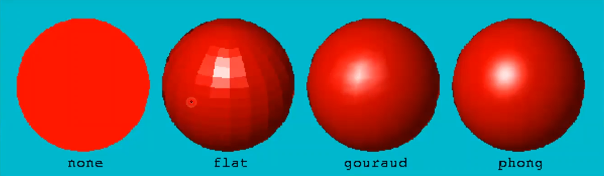
glShadeModel(GL_FLAT)glShadeModel(GL_SMOOTH)A sphere can be broken into $n$ latitudinal lines and $2m$ longitudinal lines. each polygon formed by intersecting two adjacent longitudinal lines and two adjacent latitudinal lines share a normal in flat shading.
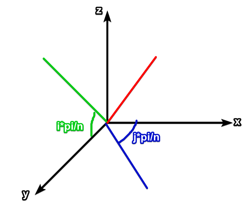
Note: point on sphere on lines $(i,j)$ ($i$ is latitude, $j$ is longitude) has \(p = \left[ \begin{matrix} r\sin(i\pi/n)\cos(j\pi/m) \\ r\cos(i\pi/n)\cos(j\pi/m) \\ r\sin(j\pi/m) \end{matrix} \\ \right]\)
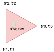
The forward mapping (texture to screen) involves:
There also is a different implementation using inverse mapping: given pixel $(x_s, y_s)$, lookup the pixel’s pre-image in texture space. This is more suitable for polygon-based raster graphics, and is the implementation in OpenGL.
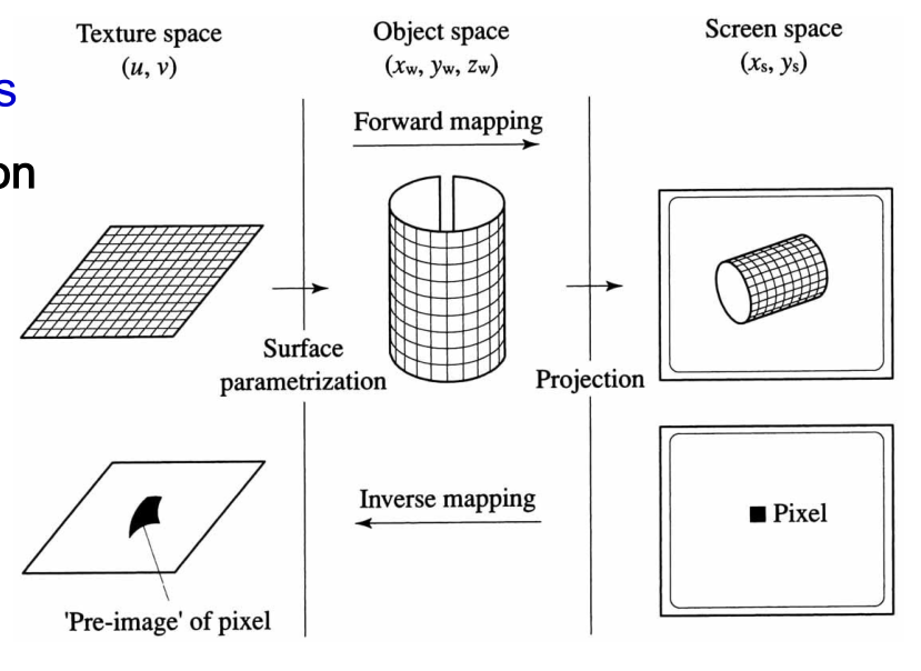
Defines surface point to texel mapping: $(x,y,z) \leftrightarrow (s,t)$. (Range of texture coordinates $(s,t) \in [0, 1]^2$.)
Per polygon, only the vertices coordinates’ mappings are specified (the rest are interpolated by the rasterizer), either manually (for complex objects), or via two-part texture mapping (for simple objects).
Two-part texture mapping involves:
S-mappings include mappings to plane, cylinder, sphere etc.
O-mappings include:
| Mapping | Description |
|---|---|
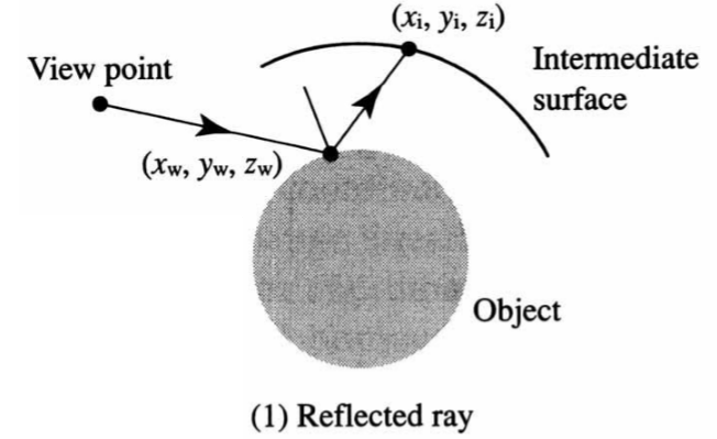 |
Dependent on view vector. Useful for environment mapping. |
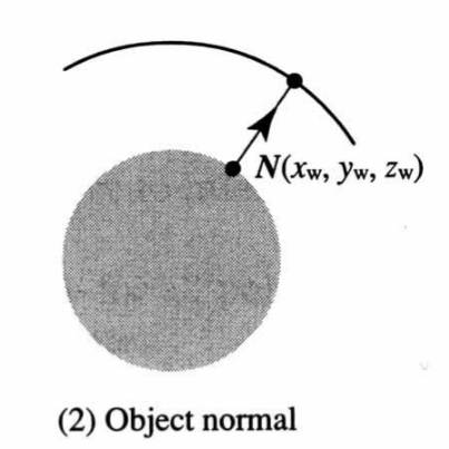 |
Ray from surface point along object surface normal |
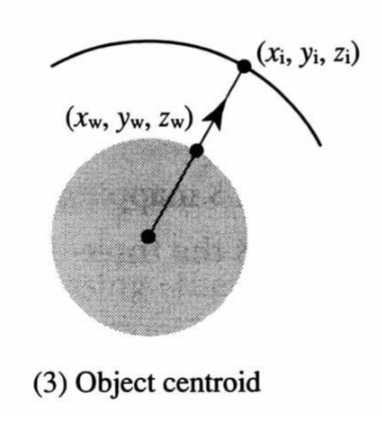 |
Ray from center through surface point |
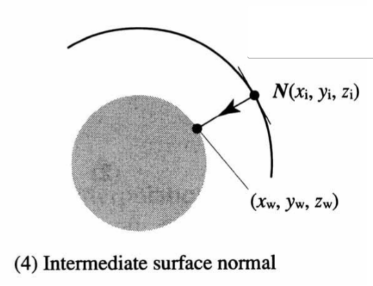 |
Ray from intermediate surface point through object surface point |
Pre-image is the texture area that the fragment maps to in texture space.
For each texture coordinate $(s, t)$ we can get:
| Interpolation in a triangle polygon | Interpolation of 4 texels |
|---|---|
 |
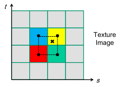 |
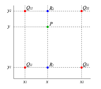
Texture filtering: determine the texture color of a fragment using the colors of the nearest 4 texels. May be implemented via bilinear interpolation.
Performing bilinear interpolation:
Clamp: $wrap(u, v) = (|u|, |v|)$
Repeated (useful for tiling): $wrap(u, v) = (u\ \% \ 1.0, v\ \% \ 1.0)$
Can happen due to:
By area-sampling each fragment, and then averaging the color that it is mapped to in the texture space.
Mipmapping: By pre-filtering texture maps, makes AA real-time performance-friendly. Successively averages each 2x2 texels until size = 1x1. Mipmap Level 0 is the original image, and Mipmap Level $\log(n)$ is the 1x1 map. (“Level”: level of texture minification.)
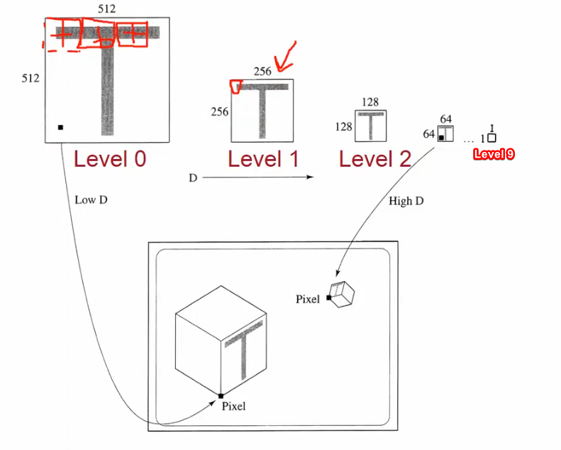
Selecting mipmap levels: If pre-image corresponds to $n^2$ texels we choose Mipmap Level $\lfloor \log n \rfloor$.
Or in the case of trilinear texture map interpolation, we interpolate between $\lfloor \log n \rfloor$ and $\lceil \log n \rceil$.
Shortcut to rendering shiny objects:
Drawbacks compared to raytracing
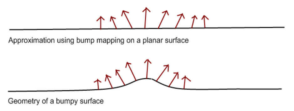
Provides a set of normals to offset the real surface’s normals by for use during lighting computation.
The texture plane is always rotated to face the view ray. (Imagine the billboards turning to face you however you turn.)
Fragment processing stage: the fragment color can be modified by texture application, mapped via texture access (using interpolated coordinates).
| Function | Task |
|---|---|
glGenTextures(int n, uint* textures) |
Creates $n$ textures, puts ids in textures. |
glBindTextures(enum target, uint texture) |
Binds texture to target. |
glTexParameteri(enum target, enum pname, int param) |
Sets parameter of target. |
glTexEnvf(enum target, enum pname, const float* params) |
Texture environment specification. i.e. How should target texture be applied onto fragment? |
void init(void) {
    // Specifies memory alignment of each pixel, 1 -> byte-alignment.
    glPixelStorei(GL_UNPACK_ALIGNMENT, 1);
    glGenTextures(1, &texObj);
    glBindTexture(GL_TEXTURE_2D, texObj);

    glTexParameteri(GL_TEXTURE_2D, GL_TEXTURE_WRAP_S, GL_REPEAT);
    glTexParameteri(GL_TEXTURE_2D, GL_TEXTURE_WRAP_T, GL_REPEAT);
    // GL_LINEAR: 4 nearest texel interpolation. not mipmapped.
    glTexParameteri(GL_TEXTURE_2D, GL_TEXTURE_MAG_FILTER, GL_LINEAR);
    glTexParameteri(GL_TEXTURE_2D, GL_TEXTURE_MIN_FILTER, GL_LINEAR);

    // Maps texture image onto each primitive active for texturing.
    glTexImage2D(GL_TEXTURE_2D, 0, GL_RGBA, imageWidth, imageHeight, 0, GL_RGBA, GL_UNSIGNED_BYTE, texImage);
}

void display(void) {
    // Activates texturing
    glEnable(GL_TEXTURE_2D);
    // how texture values are applied to the fragment
    glTexEnvf(GL_TEXTURE_ENV, GL_TEXTURE_ENV_MODE, GL_DECAL);
    glBindTexture(GL_TEXTURE_2D, texObj);
    // map Texture Coordinates <-> Objects coordinates
    glBegin(GL_QUADS);
	    glTexCoord2f(0.0, 0.0); glVertex3f(-2.0, -1.0, 0.0);
    	// ...
    glEnd();
}
To generate mipmaps:
void init(void) {
    // ...
    glTexParameteri(GL_TEXTURE_2D, GL_TEXTURE_MIN_FILTER, GL_LINEAR_MIPMAP_LINEAR);
    gluBuild2DMipmaps(GL_TEXTURE_2D, GL_RGBA, imageWidth, imageHeight, GL_RGBA, GL_UNSIGNED_BYTE, texImage)
}
Upon each intersection, the object hit may continue to shoot out secondary rays that are:
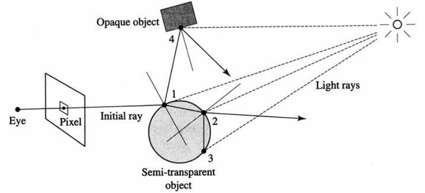
At each intersection we need to do a lighting computation and produce the reflected rays.
| Variable | Name | Task |
|---|---|---|
| $k_r$ | Reflected specular constant (0..1) | Replaces the specular constant $k_s$ |
| $k_t$ | Transmitted constant (0..1) | For transparent/translucent materials |
| $I_\text{transmitted}$ | Intensity of transmitted light | Back-propagated from the next intersection of a refracted ray |
Reflected specular: Essentially the same as the specular except that that its the reflected light, not just the highlight
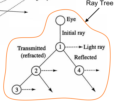
Note that this equation is recursive due to the $I_\text{reflection}$ and $I_\text{transmitted}$ values to be computed.
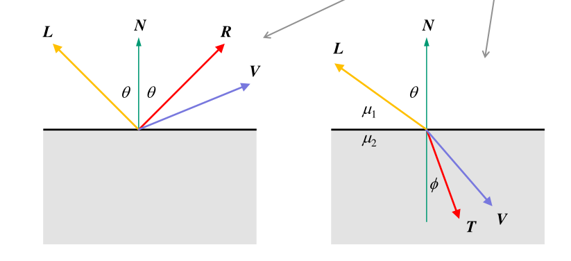
$R = 2N\cos \theta - L = 2(N \cdot L)N - L$
Snell’s law: $\mu_1 \sin \theta = \mu_2 \sin \phi$. Let $\mu = \frac{\mu_1}{\mu_2}$, then
\[\begin{aligned} T &= -\mu L + \left( \mu(\cos\theta) - \sqrt{1 - \mu^2(1-\cos^2\theta)} \right)N \\ &= -\mu L + \left( \mu(N \cdot L) - \sqrt{1 - \mu^2(1-(N \cdot L)^2)} \right)N \end{aligned}\]$k$ levels of recursion = $k$ reflection/refraction vectors in this case (i.e. 0 levels of recursion means eye to object ray only.) \(\begin{aligned} I &= I_{\text{local}, 0} + I_{\text{reflected}, 0} + I_{\text{transmitted}, 0} \\ &= I_{\text{local}, 0} + I_{\text{local}, 1} + I_{\text{reflected}, 1} + I_{\text{local}, 1} + I_{\text{transmitted}, 1} \\ &= \dots \end{aligned}\)
Shoot another ray from view ray’s intersection point towards the light source to tell if that spot is illuminated.
Hence shadow constant turns the diffuse, specular and transmitted values on or off.
Only need to find one opaque occluder to determine occlusion.
gluLookAt Camera position and orientation (World frame)gluPerspective without near and far (FOV)Image resolution: (pixels per dimension)
Ray = $P(t) = O(x,y,z) + t(\text{direction}(x,y,z))$
For the following primitives, substitute $p = O(x,y,z) + tD$ in and find $t$.
Plane = $Ax + By + Cz + D = 0 \Rightarrow N \cdot p + D = 0$ for point $p$ on plane
Sphere = $x^2 + y^2 + z^2 - r^2 = 0 \Rightarrow p\cdot p - r^2 = 0$ for point $p$ from sphere origin.
Axis-aligned box (AABB):
Triangle (polygon): Using the barycentric coordinates method
$P = \alpha A + \beta B + \gamma C = \textcolor{limegreen}{A + \beta (B - A) + \gamma (C - A)}$ where $\alpha + \beta + \gamma = 1$ and $0 \leq \alpha, \beta, \gamma \leq 1$.
\[\begin{aligned} O+ \textcolor{royalblue}{t}D &= A + \textcolor{royalblue}{\beta} (B - A) + \textcolor{royalblue}{\gamma} (C - A) \\ A - O &= \textcolor{royalblue}{\beta} (A - B) + \textcolor{royalblue}{\gamma} (A - C) + \textcolor{royalblue}{t}D \\ \left[ \begin{matrix} A_x - O_x \\ A_y - O_y \\ A_z - O_z \\ \end{matrix} \right] &= \left[ \begin{matrix} \beta (A_x - B_x) + \gamma (A_x - C_x) + tD_x \\ \beta (A_y - B_y) + \gamma (A_y - C_y) + tD_y \\ \beta (A_z - B_z) + \gamma (A_z - C_z) + tD_z \\ \end{matrix} \right] \\ &= \left[ \begin{matrix} (A_x - B_x) & (A_x - C_x) & D_x \\ (A_y - B_y) & (A_y - C_y) & D_y \\ (A_z - B_z) & (A_z - C_z) & D_z \\ \end{matrix} \right] \left[ \begin{matrix} \beta \\ \gamma \\ t \\ \end{matrix} \right] \\ & \text{can be solved with Cramer's rule.} \end{aligned}\]Note: the centroid of a triangle is located at $p = \frac{1}{3} (A+B+C)$
General polygon:
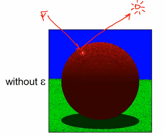
Due to floating point errors, the intersection may be “slightly below the surface”. This leads to self occlusion during shadow feeling. Methods to deal with it:
$\epsilon$ is based on the floating point accuracy.
Hard shadows only. $k_\text{shadow} \in {0,1}$
Inconsistency between highlights and reflections:
a. Light: Phong Illumination Model
b. Shadow: Shadow ray reflection
Aliasing (jaggies). each area either intersects or doesn’t.
Computes only some kinds of light transports. Doesn’t include:
Rasterization converts primitives to pixels
Raytracing converts pixels to primitives
Curves $p$ in 2D/3D, and their tangents $p’$: 1 parameter $u$.
\[p(u) = \left[ \begin{matrix} x(u) \\ y(u) \\ z(u) \end{matrix} \right], \quad p'(u) = \left[ \begin{matrix} x'(u) \\ y'(u) \\ z'(u) \end{matrix} \right]\]Surfaces $p$ in 3D, and their normals: 2 parameters $u,v$.
\[p(u,v) = \left[ \begin{matrix} x(u,v) \\ y(u,v) \\ z(u,v) \end{matrix} \right], \quad \vec{n} = \frac{\partial p(u,v)}{\partial u} \times \frac{\partial p(u,v)}{\partial v}\]Parametric curves are not unique. But they are the most used because they fit the criteria here (and are easy to render too). Note on stability: not generally true, but holds for lower degree polynomials.
For curve segments in 2D/3D, bound by $u$ and represented as:
\[p(u) = \left[ \begin{matrix} x(u) \\ y(u) \\ z(u) \end{matrix} \right] = \sum_{k=0}^n u^k\left[ \begin{matrix} c_{x,k} \\ c_{y,k} \\ c_{z,k} \end{matrix} \right] \quad \text{where $c_{\_, k}$ are constants, and } u\in[0, 1].\]For surface patches in 3D, bound by $u$ and represented as:
\[p(u) = \left[ \begin{matrix} x(u) \\ y(u) \\ z(u) \end{matrix} \right] = \sum_{j=0}^n\sum_{k=0}^n u_j v_k\left[ \begin{matrix} c_{x,j,k} \\ c_{y,j,k} \\ c_{z,j,k} \end{matrix} \right] \quad \text{where $c_{\_, k}$ are constants, and } u\in[0, 1].\]You can obtain $p$ via matrix multiplication as such, where $c = [c_{x,k} \quad c_{t,k} \quad c_{x,k}]^T$.
\[p(u) = \left[ \begin{matrix} 1 & u & u^2 & u^3 \end{matrix} \right] \left[ \begin{matrix} c_0 \\ c_1 \\ c_2 \\ c_3 \end{matrix} \right] = u^{T}c\]In practice we specify curve segments geometrically with control points.
| Type | Polynomial constraints |
|---|---|
Curve segment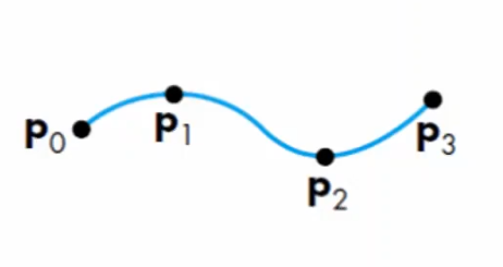 |
$p(0) = p_0$ $p(1/3) = p_1$ $p(2/3) = p_2$ $p(1) = p_3$. |
Surface patch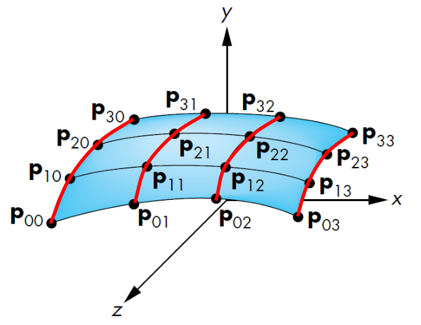 |
Interpolate the points along each red curve respectively. |
Blending functions interpolate in a way that satisfies exactly its variations along the edges of a square domain, graphical representation below.
where $v = [1 \quad v \quad v^2 \quad v^3]^T$. Note that the interpolating patch does not use the blending functions.
| Type | Illustration |
|---|---|
| $C^0$ parametric continuity (also $G^0$): |
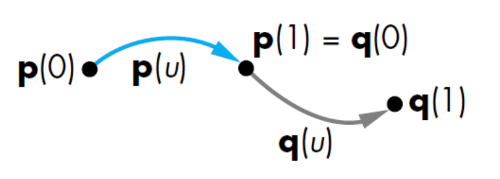 |
| $C^1$ parametric continuity | 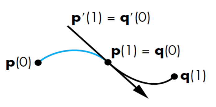 |
| $G^1$ geometric continuity | $p’(1) = \alpha q’(0)$ for some $\alpha > 0$ i.e. $p’(1)$ is parallel to $q’(0)$ |
| $C^2$ parametric continuity | $p”(1) = q”(0)$ |
Generally we have
A Bezier curve of degree $n$ is a linear interpolation of 2 corresponding points in Bezier curves of degree $n-1$. A Bezier curve of degree $n$ has $n$ control points $P_0, P_1, \dots, P_n$:
As such a Bezier curve of degree $n$ has $B’(0) = n(p_1-p_0), B’(1) = n(p_n-p_{n-1})$.
| Type | Polynomial constraints |
|---|---|
Curve segment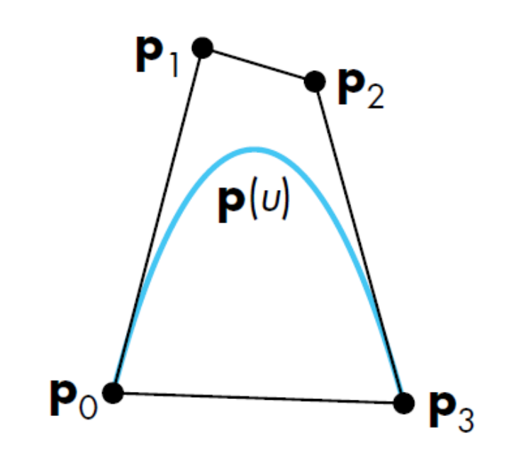 |
$p(0) = p_0$ $p(1) = p_3$ $p’(0) = 3(p_1 - p_0)$ $p’(1) = 3(p_3 - p_2)$ |
Surface patch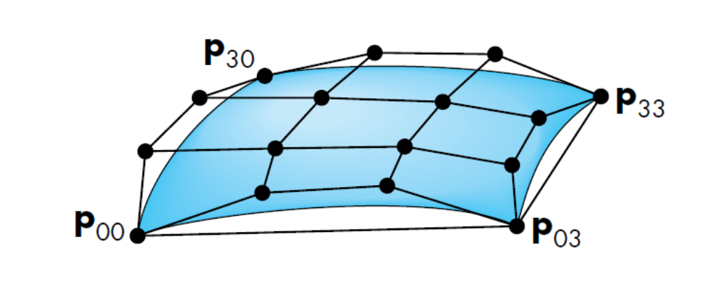 |
Interpolate the points along each red curve respectively. |
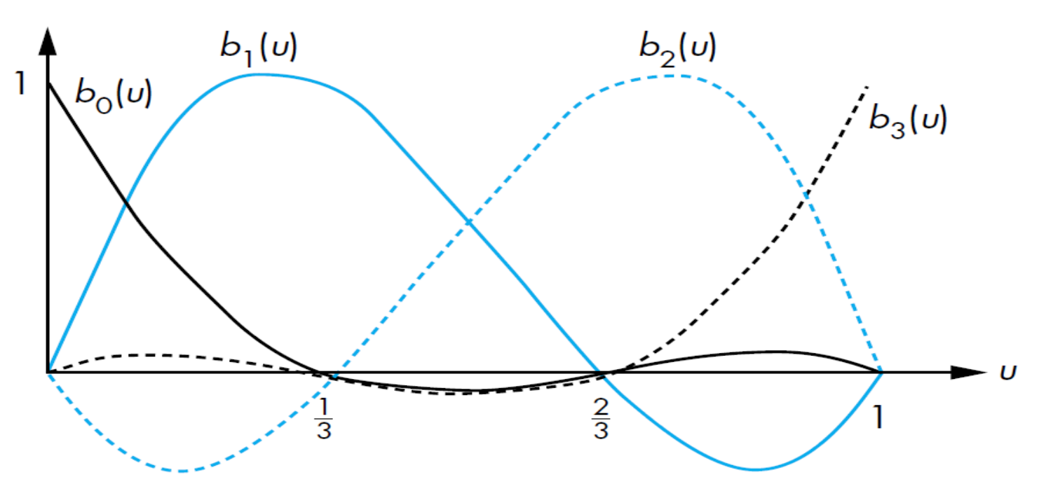
Blending functions of the cubic Bezier graph are also called Bernstein polynomials (of degree 3). For $0 \leq u \leq 1$, they satisfy:
The below shows the Bernstein polynomials. Note that the sum $p(u) = \sum_i b_i(u)p_i$ is a convex sum, and the curve is contained in a convex hull.
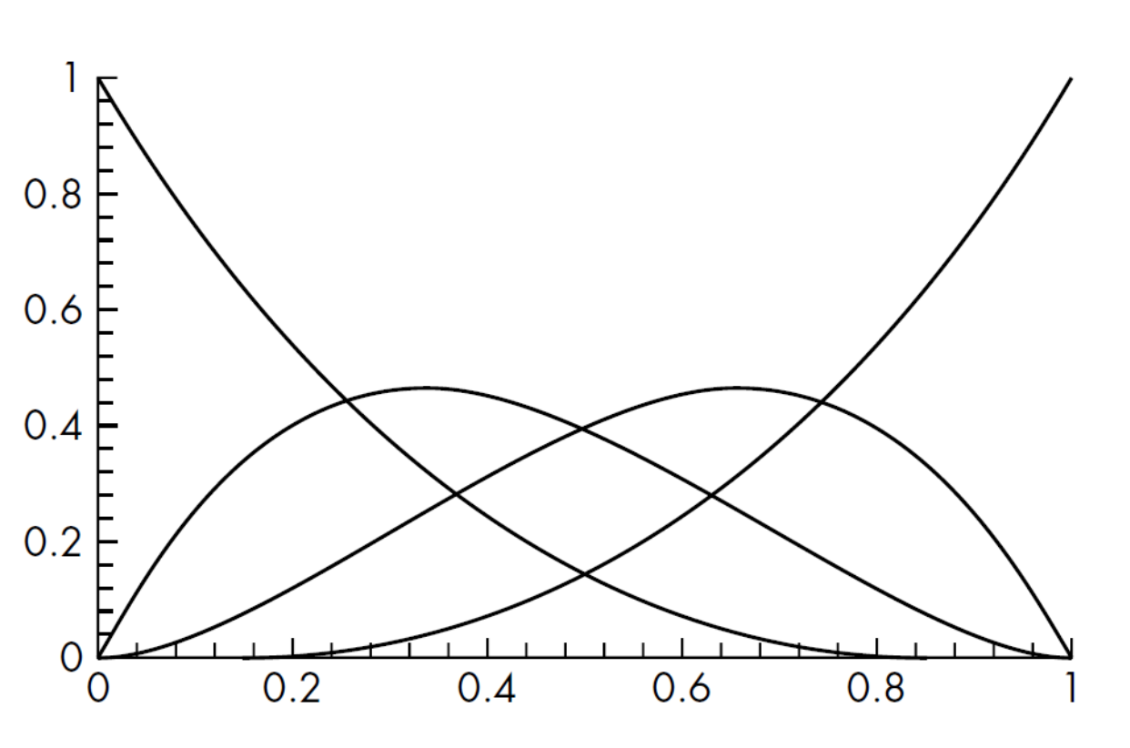
where $v = [1 \quad v \quad v^2 \quad v^3]^T$. Note that the Bezier patch uses the blending functions.
Long polynomial curves involve $\leq 4$ join points. To evaluate $p(u)$ at a sequence of join points $u_k$, use Horner’s method:
\(p(u) = c_0 + u(c_1 + u(c_2 + u(\dots +c_n)))\)
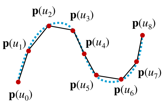
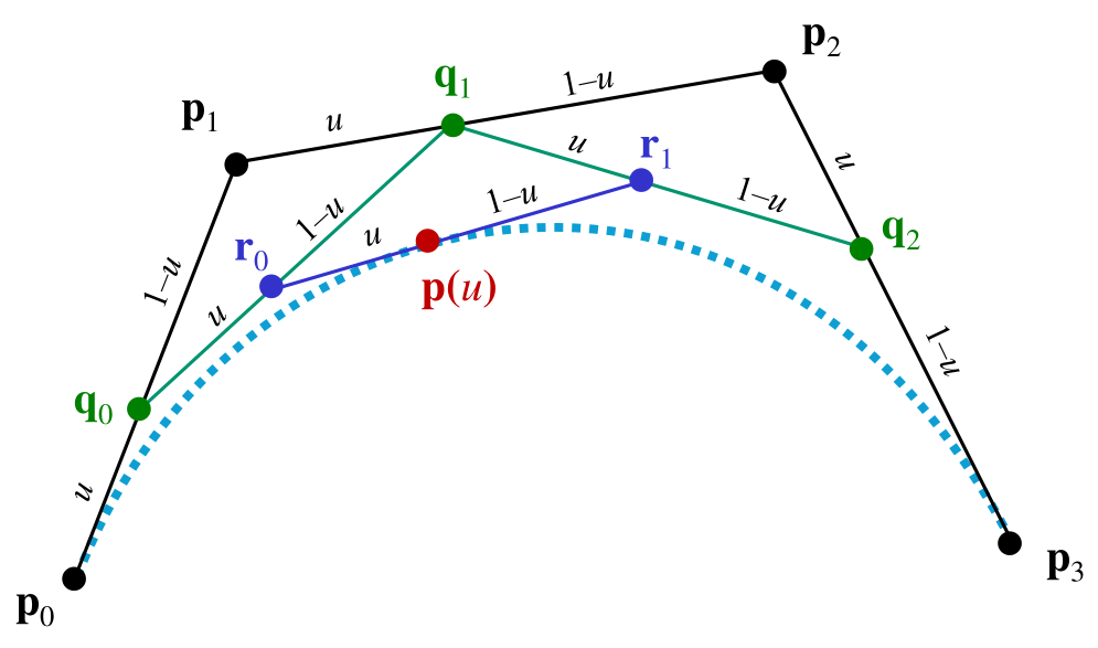
De Casteljau’s algorithm: Consecutive control points are recursively interpolated over $u \in [0, 1]$, in the case of the curve.
| Bezier curves $p$ | Interpolating curves $q$ |
|---|---|
| known $c \rightarrow$ find unknown control points $p$ | known $c \rightarrow$ find unknown control points $q$ |
| known $p \rightarrow$ find unknown $c$ | known $q \rightarrow$ find unknown $c$ |
| Simple blending functions ($M_B$) | Rather messy blending functions ($M_I = u^TA^{-1}$) |
| Includes $M_B$ in bezier patch | Doesn’t include $M_I$ in interpolation patch |
