2 forms of rendering equations: Hemispherical and Area formulations.
Hemispherical: Integrates incoming radiance from the hemisphere around point $x$.
Area: Integrates incoming radiance from all surfaces in the scene. (Involved in radiosity computation).
Involves sending many rays, so it cannot be computed analytically. Instead can use iterative methods such as MCRT below.
| Partial Global Illumination | Global Illumination |
|---|---|
Whitted Raytracing LD?S*E |
Path tracing L(D|S)*E |
Distribution Raytracing LD?S*E |
Two-pass ray tracing LS+DS*E |
Radiosity LD*E |
Photon-mapping LS+DS*E |
Monte Carlo techniques for solving integrals without analytic solution.
Algorithms are:
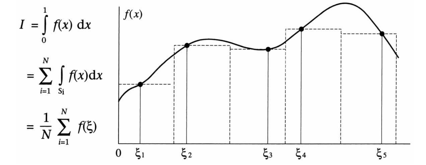
Generates random samples of integrand and averages the result.
\[\begin{aligned} I &= \int_a^b f(x) dx \\ &\approx \frac{b-a}{N} \sum^N_{i=1} f(\xi _i) \\ &= I_m \end{aligned}\]Note that $\lim_{N \rightarrow \infty} I_m = I$.
For $N$ uniformly distributed random samples,
\[\left| I_m - I \right| = \frac{k}{\sqrt{n}}\]Sample once per stratum (an equally sized subregion).
Error reduced to $k/N$.
Sampling values with higher probabilities.
Works with knowledge of material’s BRDFs.
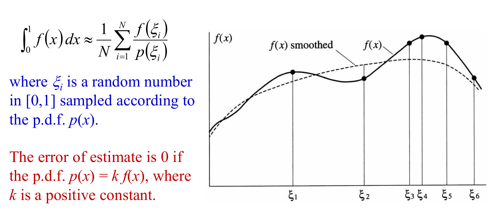
Problem: Hard to know the sampling distribution (even with BRDF) beforehand (e.g. caustics).
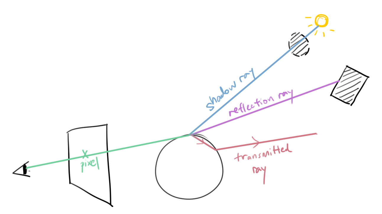
LD?S*ESee previous chapter.
Same as Whitted ray tracing except all specular paths are calculated.
View dependent, partial global illumination.
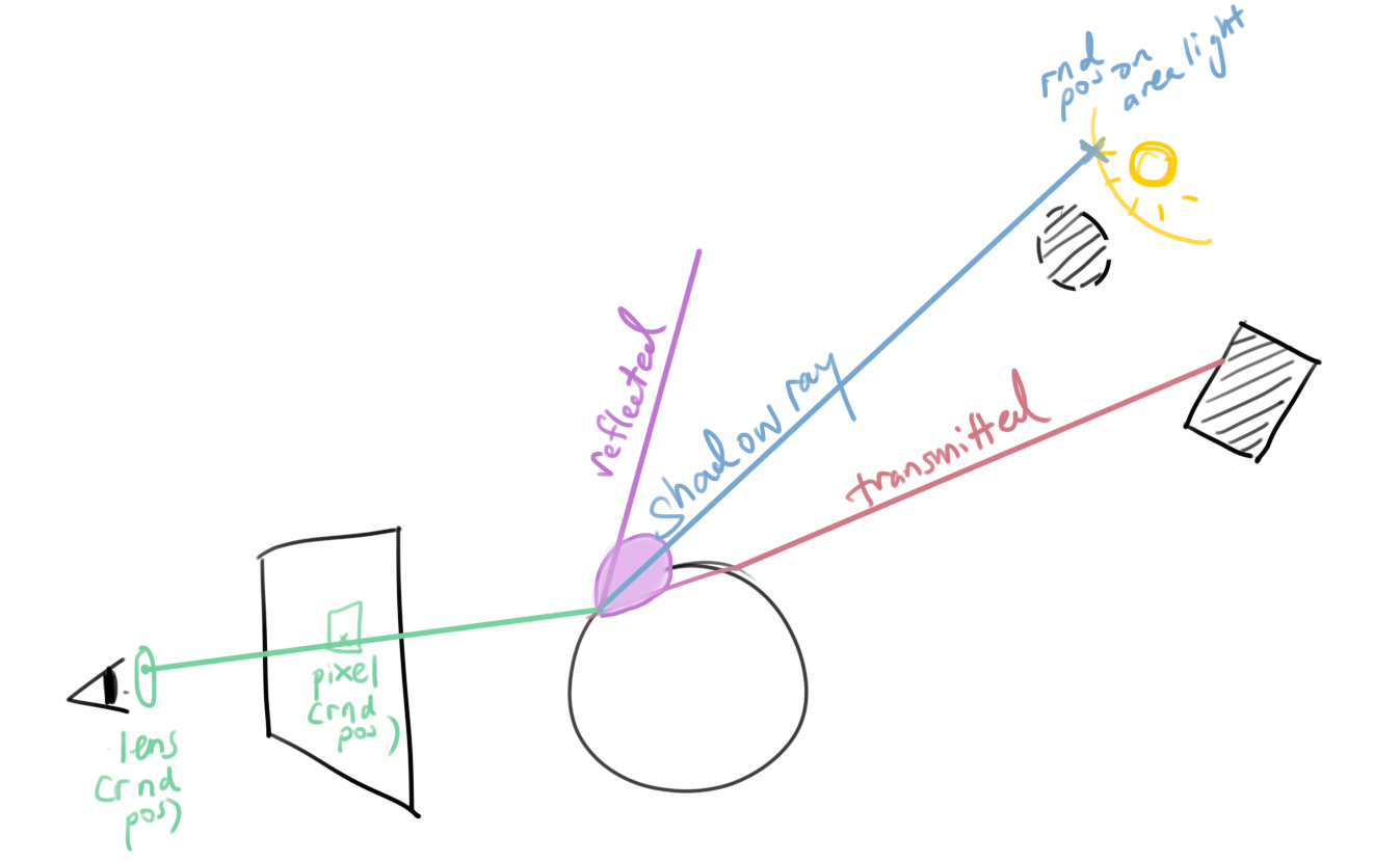
L(D|S)*EView dependent, complete global illumination.
High computational cost: Needs to shoot many paths per pixel to reduce noise.
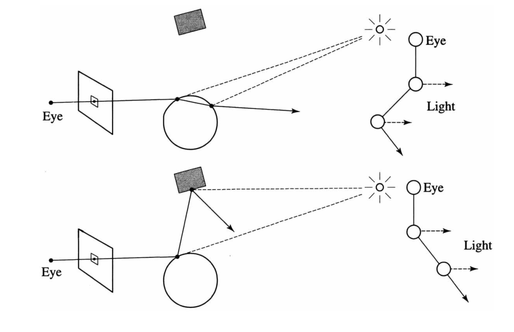
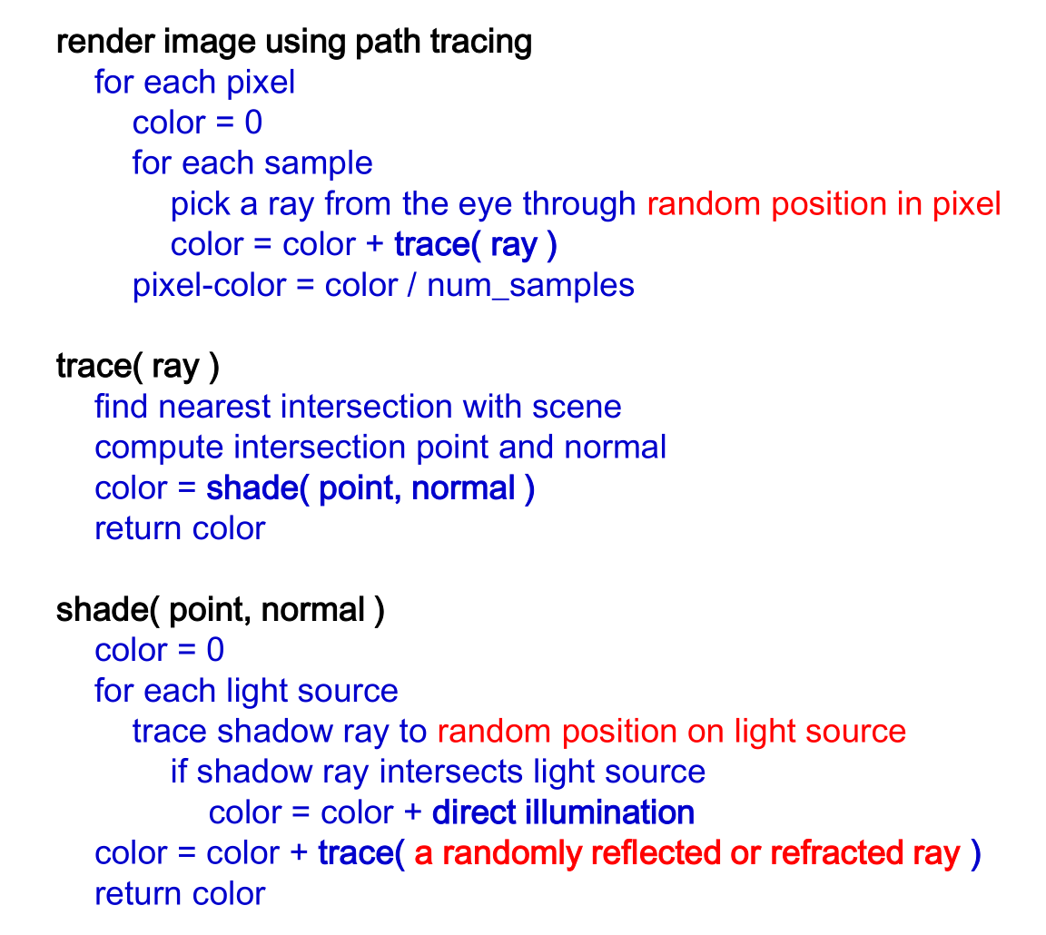
This happens due to lack of control over in which direction does the traced reflection/refraction ray shoot toward.
LS*DS*ERays shot from light source (light “view”) and stored in lightmap, requires surface parameterization.
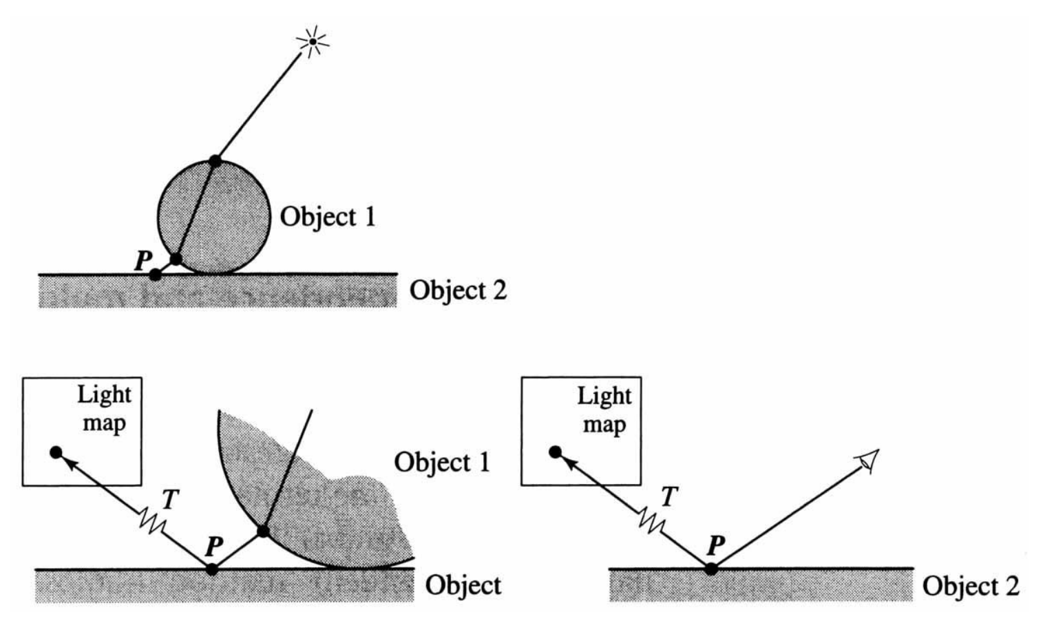
LS*DS*EPhotons shot from light source (light “view”) and stored in lightmap.
Key-value pair: Photon map values, unlike in light map, are stored with respect to a 3D position vector. Includes
Data structure is kd-tree: Efficient for querying $k$ closest photons about any 3D locaiton (for estimating outgoing radiance per surface point)
| Rendering value | Explanation | Example |
|---|---|---|
| Direct illumination | Shadow ray |  |
| Specular reflection | Specular/glossy reflections |  |
| Caustics | Caustics photon map |  |
| Indirect illumination | Tracing secondary rays to photon map |  |